Solving Lambert’s Problem, Part I: Foundations Through Kepler and Geometry
Introduction
Welcome. This post lays the foundation for solving Lambert’s Problem in orbital mechanics—a cornerstone question in mission planning and trajectory design.
The Core Question:
Given the position of a celestial body at two distinct times, can we determine the orbit it followed?
More formally: Can we determine the conic section (typically an ellipse) defined by two position vectors and the time of flight between them?
This is Part I of a two-part series. Here, we focus on the physical intuition, Keplerian time relationships, and the geometric structure behind Lambert’s Problem. In Part II, we’ll derive and apply the full Lambert formulation.
Kepler’s Equation
A key component in solving Lambert’s Problem is Kepler’s Equation, which links time of flight to position via orbital anomalies:
$$ M = E - e\sin E \tag{1} $$Where:
- \( M \) = Mean Anomaly
- \( E \) = Eccentric Anomaly
- \( e \) = Eccentricity
Mean Anomaly: Think of it as the angular position the body would have if it were moving uniformly in a circular orbit with the same period.
Eccentric Anomaly: The projection of the body’s true position on the auxiliary circle that circumscribes the ellipse. Eccentric anomaly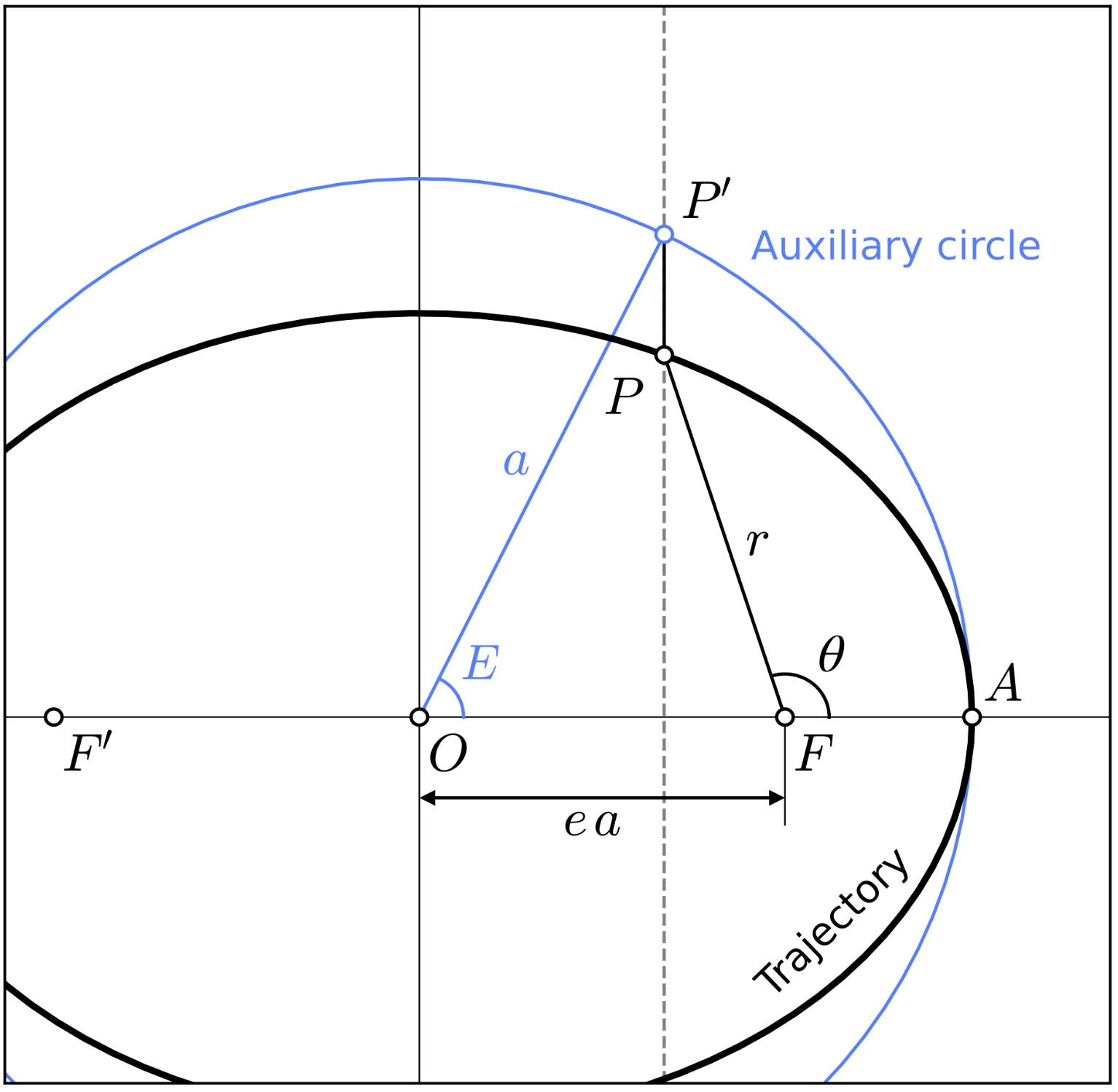
Eccentricity: A measure of how much an orbit deviates from circularity.
- \( e = 0 \) → perfect circle
- \( 0 < e < 1 \) → ellipse
See more on eccentricity
Worked Example
Let’s say we have:
- Semi-major axis \( a = 10,000 \ \text{km} \)
- \( t_1 = 0 \), \( t_2 = 2000 \ \text{s} \)
- Eccentricity \( e = 0.2 \)
Compute Mean Anomaly:
$$ M = \sqrt{\frac{\mu}{a^3}}(t_2 - t_1) $$With \( \mu = 3.986 \times 10^{14} \ \text{m}^3/\text{s}^2 \):
$$ M = \sqrt{\frac{3.986 \times 10^{14}}{(10^7)^3}} \cdot 2000 \approx 1.261 \ \text{rad} $$Time of Flight via Anomalies
To connect Kepler’s Equation to Lambert’s framework, we subtract two time-position relations:
$$ M = E - e\sin E $$Subtracting between two points:
$$ M_2 - M_1 = (E_2 - e\sin E_2) - (E_1 - e\sin E_1) $$Now replace Mean Anomaly with time:
$$ \sqrt{\frac{\mu}{a^3}}(t_2 - t_1) = (E_2 - e\sin E_2) - (E_1 - e\sin E_1) $$This is the first key equation: it expresses the time of flight purely in terms of eccentric anomalies.
Radius and Eccentric Anomaly Relationship
We want to move from anomaly-based expressions to ones based on known quantities like position vectors. This helps later when we don’t know the anomalies.
A key identity:
$$ r = a(1 - e\cos E) $$This connects radius \( r \) at any point to the semi-major axis and eccentric anomaly.
📘 For full derivation, see:
Prussing, J. E., & Conway, B. A. (2013). Orbital Mechanics (2nd ed.). Oxford University Press. Section 2.2, p. 28.
A Transcendental Form of Lambert’s Equation
Using:
$$ \sqrt{\frac{\mu}{a^3}}(t_2 - t_1) = (E_2 - e\sin E_2) - (E_1 - e\sin E_1) $$And replacing each \( E \) using:
$$ E = \cos^{-1} \left(\frac{a - r}{ae}\right) $$We arrive at:
$$ \begin{aligned} \sqrt{\frac{\mu}{a^3}}(t_2 - t_1) &= \left[ \cos^{-1}\left(\frac{a - r_2}{ae} \right) - e\sin\left( \cos^{-1}\left( \frac{a - r_2}{ae} \right) \right) \right] \\ &- \left[ \cos^{-1}\left(\frac{a - r_1}{ae} \right) - e\sin\left( \cos^{-1}\left( \frac{a - r_1}{ae} \right) \right) \right] \end{aligned} $$While solvable with brute force, this form is not practical. A geometric method is more insightful—and more elegant.
Geometric Constraints of the Transfer Orbit
Geometric Property of Ellipses
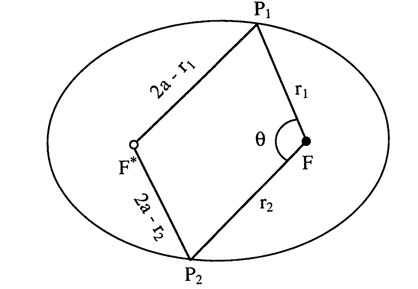
Every ellipse has two foci. For an orbit, one is occupied by the central body (e.g., Earth). The other—the vacant focus—plays a crucial role in determining the transfer orbit.
The ellipse obeys a key property:
The sum of distances from any point on the ellipse to the two foci equals \( 2a \), the major axis length.
So:
$$ P_1F + P_1F' = 2a $$Or more concretely:
$$ r_1 + (2a - r_1) = 2a $$You can visualize this with:
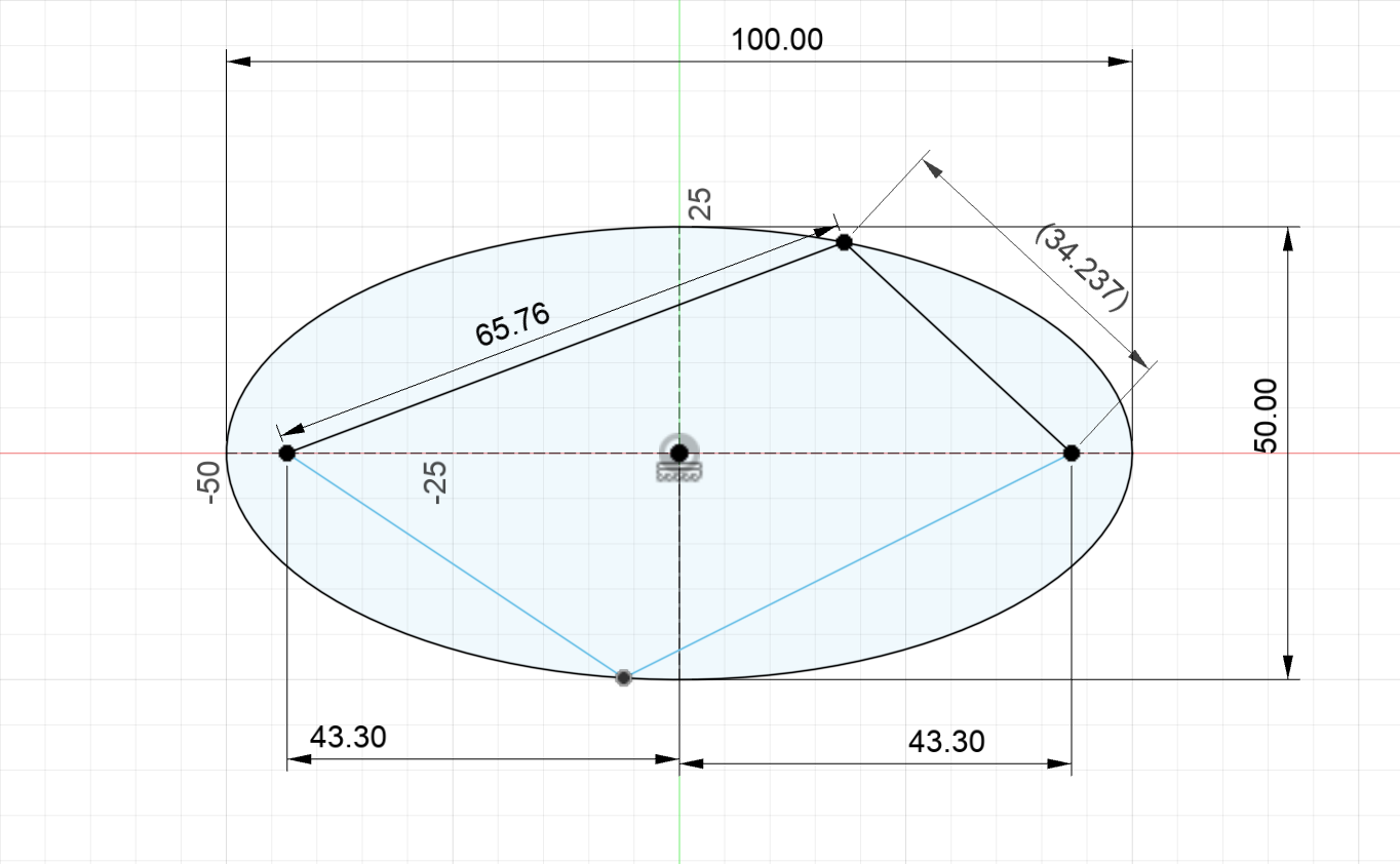
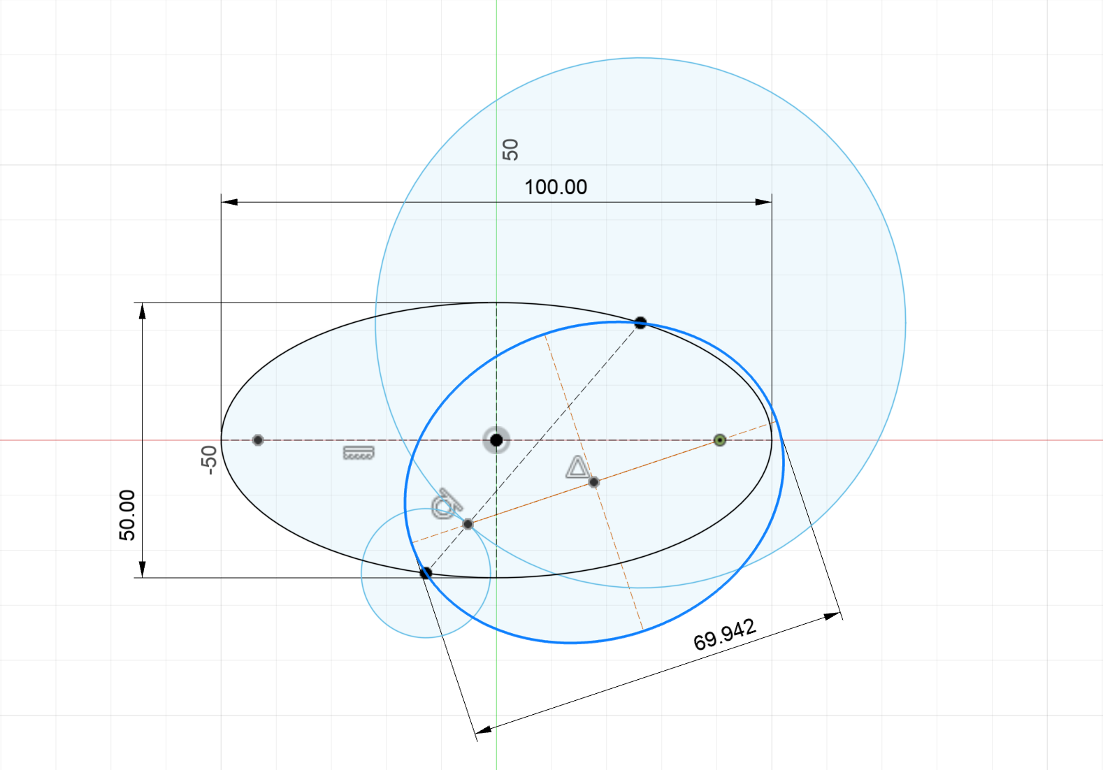
Geometric proof of ellipses using design software.
Now consider how we locate that second focus geometrically. If we fix points \( P_1 \) and \( P_2 \), and draw circles of constant radius from them, the intersections of those circles represent potential positions for the vacant focus. Each such point defines a valid elliptical transfer.
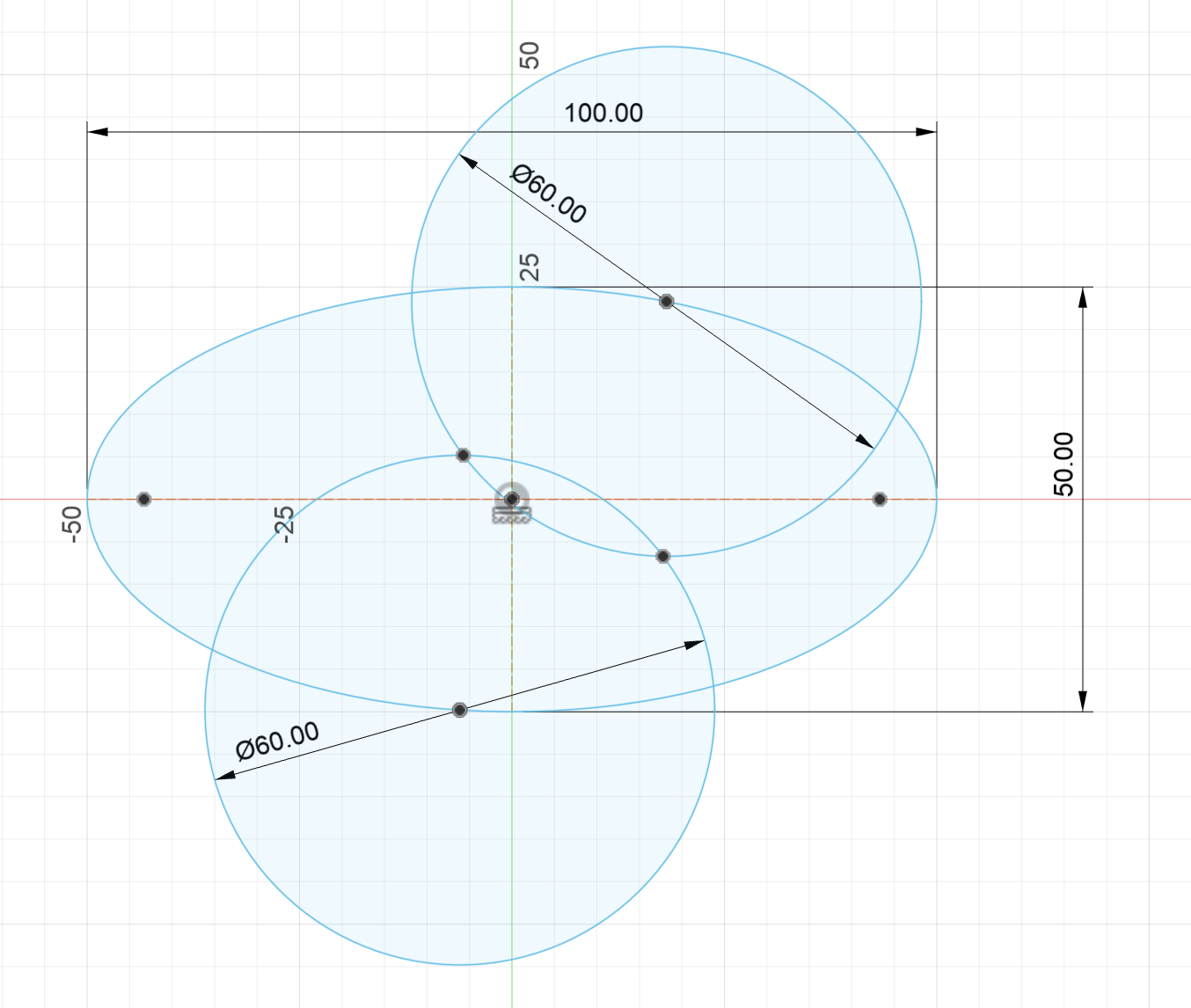
Search for semi-major axis via geometric intersections.
At each intersection, there exists a possible ellipse passing through \( P_1 \) and \( P_2 \) with the appropriate focal configuration.
When the two circles touch at exactly one point, this corresponds to the minimum energy transfer orbit.
Optimal energy transfer orbit when vacant focus lies on P1-P2 chord.
This orbit requires the least delta-v, but not necessarily the shortest time. Among all transfer orbits satisfying Lambert’s constraints, the most circular one (least eccentric) tends to be the most efficient energetically.
Why the Vacant Focus Lies on the Chord
The minimal-energy ellipse has its secondary focus lying directly on the chord connecting \( P_1 \) and \( P_2 \). This minimizes the ellipse’s eccentricity and thus the required velocity change.
In Part II, we’ll use this geometric constraint, combined with orbital mechanics principles, to derive the full Lambert formulation.
*Next: In Part II, we’ll solve Lambert’s Problem fully—deriving the final equations