BULGARIAN NATIONAL TELEVISION (BNT)
I was featured on Bulgarian National Television (BNT) in a segment focused on real-time avalanche detection and the development of AvMAP (Avalanche Detectors).
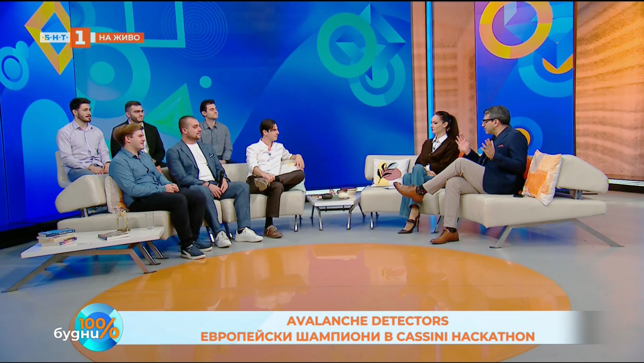
BNT live segment: Avalanche Detectors — European Champions in CASSINI Hackathon.
The feature explored how satellite Earth-observation data can be used to monitor avalanche-prone terrain and support better decision-making for mountaineers, ski resorts, and rescue services. I discussed the technical approach behind AvMAP, including the motivation for the project and its potential societal relevance in improving safety in mountainous regions.
GAS–SURFACE INTERACTIONS IN HYPERSONIC REENTRY (RAREFIED REGIME)
At extreme altitudes—above 100 km and especially in low Earth orbit (~400 km)—Earth’s atmosphere becomes so rarefied that it can no longer be treated as a continuum. Instead, the behavior of gas transitions to what is known as free molecular flow. In this regime, individual gas molecules rarely collide with one another; instead, they interact almost exclusively with the surfaces they encounter, such as the heat shield of a re-entry capsule.
RUNGE KUTTA: THE WORKHORSE NUMERICAL INTEGRATIOR FOR ORBITAL MECHANICS AND MORE
It is my goal to teach you how this numerical integratior works and hopefully why its better than the classical Euler solver you might be useto
FROM KEPLER TO CARTESIAN – CONVERTING ORBITAL ELEMENTS TO POSITION AND VELOCITY
When you’re just starting out in orbital mechanics, Keplerian elements can feel like the secret code of the cosmos: elegant, compact , they work! Six numbers that somehow capture the shape, tilt, and timing of the orbits’s path around the Earth.
You get eccentricity - telling you how circular something is
Inclination - saying what is its tilt and then some of the less intuitive ones, like the Argument of Perigee, which simply tells you at what angle along the orbit the closest point (perigee) is.
SOLVING LAMBERT’S PROBLEM, PART I: FOUNDATIONS THROUGH KEPLER AND GEOMETRY
Introduction
Welcome. This post lays the foundation for solving Lambert’s Problem in orbital mechanics—a cornerstone question in mission planning and trajectory design.
The Core Question:
Given the position of a celestial body at two distinct times, can we determine the orbit it followed?
More formally: Can we determine the conic section (typically an ellipse) defined by two position vectors and the time of flight between them?
This is Part I of a two-part series. Here, we focus on the physical intuition, Keplerian time relationships, and the geometric structure behind Lambert’s Problem. In Part II, we’ll derive and apply the full Lambert formulation.
LECTURE ON LAMBERTS PROBLEM
Background
This post contains a lecture I delivered to my colleagues at Sofia University.
Inspired by the real-world applications of Lambert’s Problem in lunar and interplanetary transfers, I structured this material to cover both the theoretical foundations and the numerical methods required to solve it. The lecture includes derivations, Kepler’s equation extensions, historical context, and a practical implementation for an Earth-to-Moon mission using a ∆V-constrained trajectory.
Key Takeaways from the Lecture
- Full derivation of Lambert’s equation from geometric and anomaly-based methods
- Historical evolution: From Lambert and Lagrange to Gauss and modern numerical solvers
- Application: Transfer trajectory planning with ∆V constraints and lunar orbit targeting
- Implementation: Code-ready parameters modeled after Apollo mission architecture
- Tools: Applied in FreeFlyer with contextual mission planning using a porkchop plot subset